Demand Prediction with LSTMs using TensorFlow 2 and Keras in Python

View the complete project on Github

One of the most common applications of Time Series models is to predict future values. How the stock market is going to change? How much will 1 Bitcoin cost tomorrow? How much coffee are you going to sell next month?

This guide will show you how to use Multivariate (many features) Time Series data to predict future demand. You’ll learn how to preprocess and scale the data. And you’re going to build a Bidirectional LSTM Neural Network to make the predictions.

Steps

1. Data
2. Feature engineering
3. Visualization and exploration
4. Preprocessing
5. Prediction
6. Evaluation

Data

Our data London bike sharing dataset is hosted on Kaggle. It is provided by Hristo Mavrodiev. Our goal is to predict the number of future bike shares given the historical data of London bike shares.

Feature engineering

Feature exploration

• - timestamp - timestamp field for grouping the data
• - cnt - the count of a new bike shares
• - t1 - real temperature in C
• - t2 - temperature in C “feels like”
• - hum - humidity in percentage
• - wind_speed - wind speed in km/h
• - weather_code - category of the weather
• - is_holiday - boolean field - 1 holiday / 0 non holiday
• - is_weekend - boolean field - 1 if the day is weekend
• - season - category field meteorological seasons: 0-spring ; 1-summer; 2-fall; 3-winter.

Our dataset is fairly clean; however, for further analysis, we are going to convert the timestamp column into a timestamp data type to extract further information (hourly, daily, monthly)

Visualization and exploration

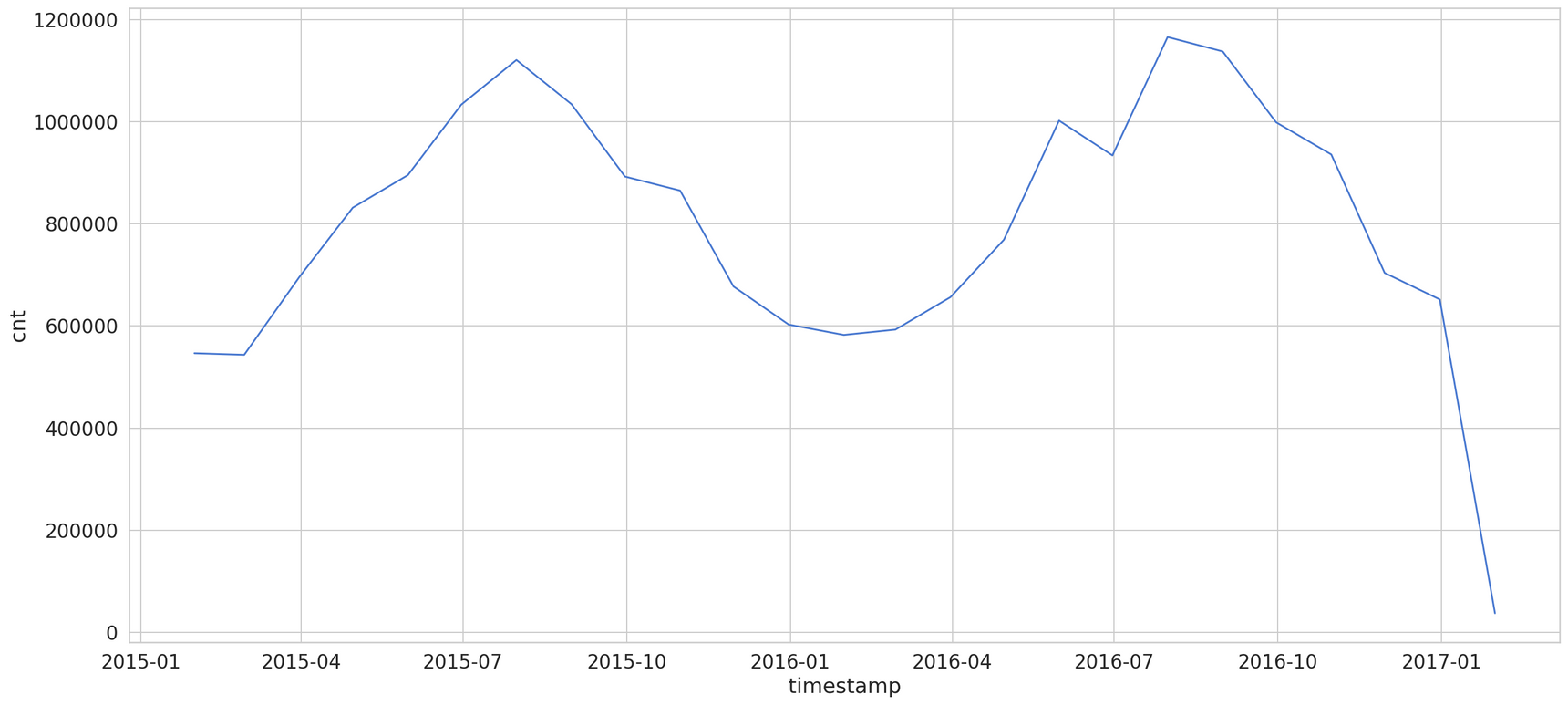
Monthly

Our data seems to have a strong seasonality component. Summer months are good for business. Throughout the 12-month period, while not many people use this service at the beginning and at the end the year (the figure is the lowest in late December - January), there is an exponential growth of users between January and September, reaching a spike in October. Therefore, it is concluded that most people favor using bike shares in the middle of the year, which is reasonable because the weather is dry and humid at this period of the year.

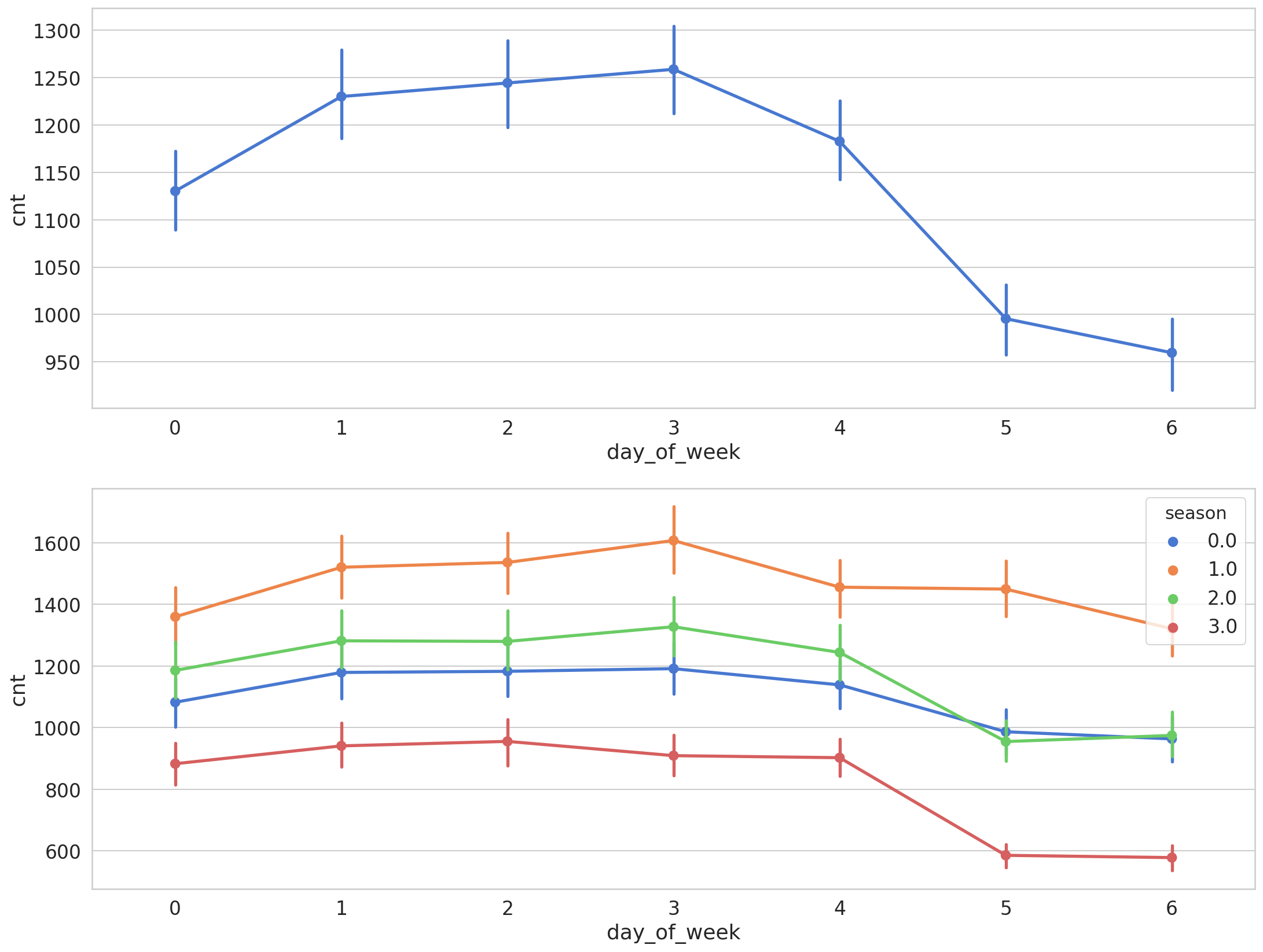
Weekly

Looking at the data by day of the week shows a much higher count on the number of bike shares.

Hourly

The hours with most bike shares differ significantly based on a weekend or not days. Workdays contain two large spikes during the morning and late afternoon hours (people pretend to work in between). It is witnessed that the majority of people at 8 A.M and 18 P.M, which coincides with the time that people commute to work. In addition, it is also notable that the figures starts to increase dramatically from 5a.m to 8 a.m, which is proved by the fact that people start to do exercise during this time. On weekends early to late afternoon hours seem to be the busiest.

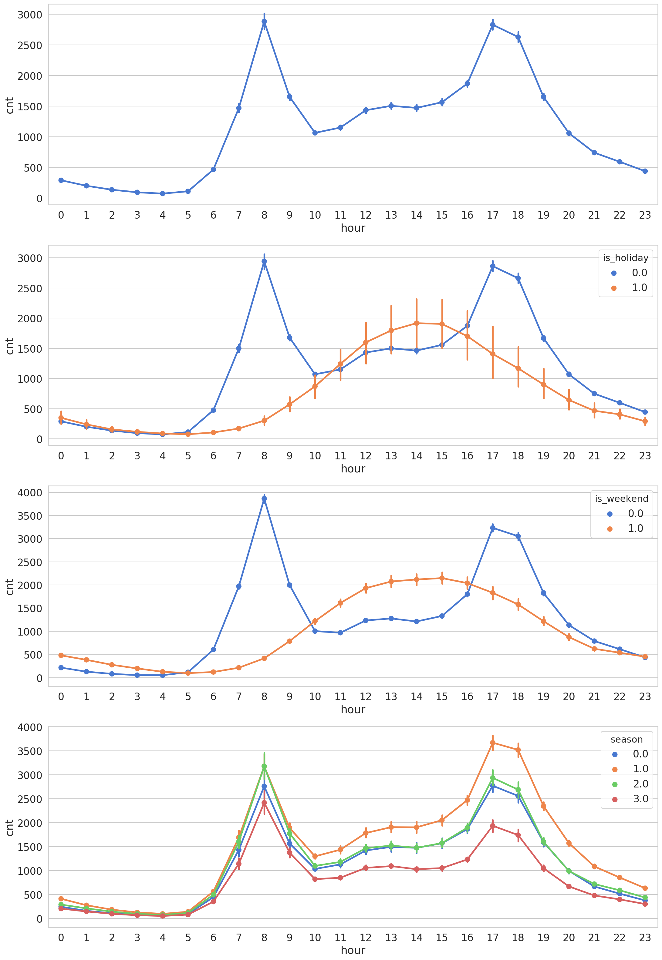
The new features separate the dataset very well.

• - Python
• - Django + Django REST Framework
• - React JS
• - Postgres
• - AWS (S3 & RDS)
• - Zingcharts - Trending & graphing test results
• - Google Maps API
• - XML2PDF - PDF generator

Preprocessing

For this dataset, 10% of the data will be used for testing, at the same time, numerical features are scaled using StandardScaler to facilitate deep learning process. All of these operations are wrapped in create_dataset() function.

In addition, a time step of 10 (10 consecutive data points will be used to predict the next one) is applied in the Bidirectional LSTM model.

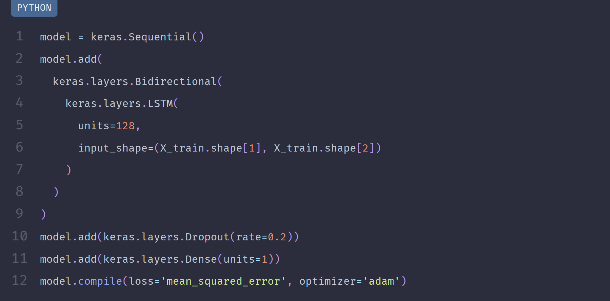
Prediction

By the time I am writing this article, I am still a beginner to time series forecasting; therefore, further upgrade on the model should be made later. But first, let’s start with a simple model and see how it goes: One layer of Bidirectional LSTM with a Dropout layer

Evaluation

Here’s what we have after training our model for 30 epochs:

The model converges pretty fast, at about epoch 5, it is already starting to overfit a bit. This is our prediction for the last 100 time steps

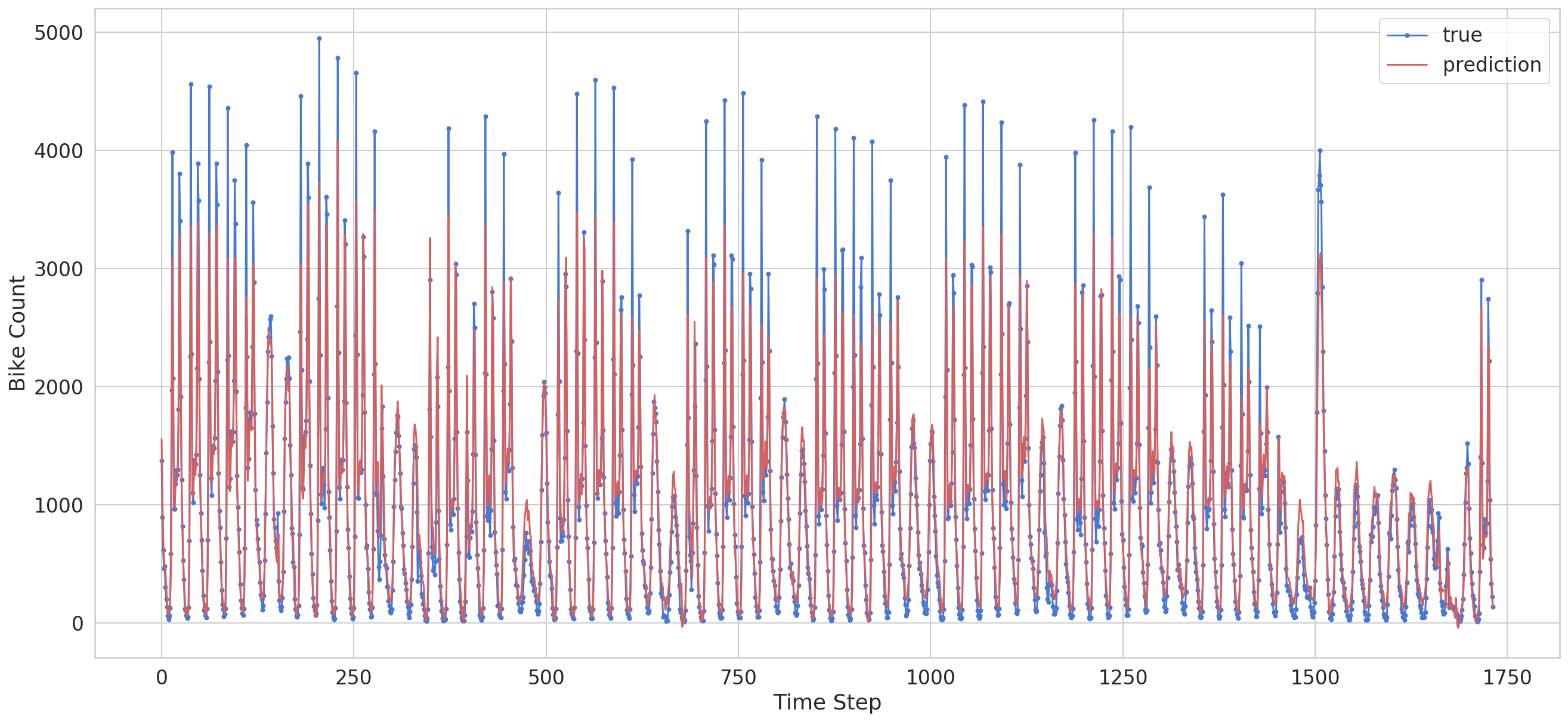
Note that our model is predicting only one point in the future. That being said, it is doing very well. Although our model can’t really capture the extreme values it does a good job of predicting (understanding) the general pattern.